Постройте сначала хоть какую-то. Далее научитесь делать группировку по датам:
Группировка данных в сводной таблице
Хотя сразу видно нестыковки какие-то в предлагаемом формате. У поволжья одновременно два итога(вверху и внизу), а это некорректно. Плюс в столбцах не для всех полей присутствуют месяцы — так в сводной не сделать.
Хотя…Исходные данные какие-то…Мягко говоря уродские для сводной. Есть подозрение, что все что от Вас требуется это убрать объединенные ячейки и при помощи сводной тупо разбить на Дивизион и Наименование. Остальные данные взять из одноименных столбцов.
Getting the Pivot table field name is not valid error message while trying to create a pivot table or while performing any operation on the pivot table?
Don’t get worried as this post will help you out to get complete information about PivotTable field name is not valid error and ways to fix it off.
[cta-excel-repair-lite labl=”retrieve lost Excel data”]
Microsoft Excel is a very powerful and useful application of the Microsoft Office suite. But apart from its popularity and usefulness, this is a very complex application as well. Due to this reason Microsoft has offered various useful features to make the task easy for the users.
The Pivot table is one of them; this is the most powerful feature of MS Excel. It helps in extracting main information from the detailed and large datasets. This is created for tracking details to make the task easy for the users.
But many users informed that while creating the Pivot Table they come across “The PivotTable field name is not valid.” error message. The error simply states that source data is not suitable and this is the main reason for getting the error.
Here is error declaration:
“The PivotTable field name is not valid. To create a PivotTable, you must use data that is organized as a list with labelled columns. If you are changing the name of a PivotTable field, you must type a new name for the field.”

So here you need to make your data suitable for a Pivot Table or utilize data that is organized as a list with labelled columns. Make sure if you are changing the name of a Pivot Table field, then must type a new name for the field.
Apart from that, it is also possible the error appears because Excel needs a field name (column header) for indexing data in a pivot table form and with the missing field names, Excel, cannot index and utilize data.
How To Fix Pivot Table Field Name Is Not Valid Error?
Well, the error message is quite confusing as there are many reasons responsible for getting the Excel error. Users might also get the error if one or more spaces are presented in range first row where Pivot Table tries extracting data.
Microsoft has offered various working solutions to fix the error message, here follow each one.
1: Alter First Row
In this case, you need to modify the table first row in a way that it should not contain a single empty cell.
And after doing so check the error is resolved or not.
2: Modify the Range
Changing or altering range that Pivot Table mentions to a range in which the first row does not include any empty cells help you to fix MS Excel Pivot Table error message
Here check out the complete process to change the range of active Pivot Table references as shown.
- In the Pivot table > choose a cell
- Then from the data menu click on the PivotTable Report option.
- After that click on the back button will show the PivotTable Wizard
- Then in the window that shows the > current range for Pivot Table will appear> edit Source Data Range.
- Lastly, click Finish > exit the window
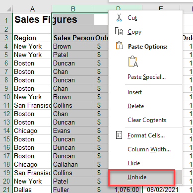
3: Unhide/ Delete Empty Columns
This is the quick fix that helps you to solve PivotTable Field Name is not Valid error.
Follow the steps to do so:
- To the left of cell A1,> click Select All button

- Then right-click any column heading > choose Unhide.

- Try to create Pivot Table again.
Hope this works for you but if not then delete empty columns as this worked for many users.
4: Fix The Field Name Issue
The error message commonly appears as one or more heading cells in source data are blank. For creating a pivot table, you require heading for each columns.
And to locate the issue, try the below-given steps:
- In creating PivotTable dialog box > check the Table/Range selection to assure you haven’t selected blank columns next to the data table.
- Or check for hidden columns in source data range > add headings whether they are missing.
- If in the heading row there are any merged cells > unmerge them > add a heading in each separate cell.
- Choose each heading cell > check its contents in formula bar > text from one heading might overlap blank cell beside it. For example, the Product Name heading overlapped empty heading cell next to it.

Tip: From your data, if you create an Excel Table, then the column headings are automatically added to columns with blank heading cells.
Hope this works for you.
5: Assign Header Value
You can’t create a pivot table without assigning the header value. All the columns having data in it must have the heading value too. If in case any cell lacks in this, then you will definitely get the pivot table error.
6: Complete Data Got Deleted
After creating the PivotTable if the entire data gets deleted. besides that you are trying to refresh the report after the data range is been deleted then it’s obvious to get the Pivot Table field not valid error message.
7: Don’t Select The Entire Sheet
General this mistake is done by the beginners. They select the complete datasheet to create pivot table, which is not the right way. Thus they encounter such type of Pivot Table errors.
8: Column Header Is Deleted
Chances are also that column header is somehow got deleted after creation of the pivot table.
If you don’t have any column header then you are not allowed to insert pivot table also.
Sometime situation also occur where at the time of pivot table creation, table header is present. But when you refresh the pivot table to update it’s table header gets deleted and thus you start getting the error.
So check for it whether your pivot table is also having the missing table header.
9: Rename Field/Item In The PivotTable
- Tap to the item or field which you needs to rename.
- Now hit the PivotTable Tools and then the Analyze option. After that from the Active Field group you need to make a tap over the text box of Active Field.

If you are a Excel 2007/2010 user then go to the PivotTable Tools > Options.
- Assign new name and hit enter button.
10: Unmerge The Merged Cell
To fix Excel Pivot table field name not valid error, the last solution that you can try is unmerging the merged cells.
- Choose entire column present within the Excel table.
- After that make right-click over the selected column and then tap to the Unhide option.
- Check for the merged cells and then unmerge it by following this path: Home >> Alignment >> Merge & Center.

Best Recovery Tool For Lost/Corrupted Excel PivotTable:
Excel Recovery software is the best tool to recover corrupted/damaged/lost Excel workbook, spreadsheet. This tool is built with advanced features for easy and quick excel document recovery. It can recover data from multiple corrupted workbook and also recover pivot table data in one go.
* Free version of the product only previews recoverable data.
So if you lost your Excel pivot table data due to Pivot table field name not valid error then don’t get panic just try this excellent recovery utility.
FAQ:
How To Insert Pivot Table On Excel?
Follow the given steps to do so:
- Inside data set > click on any single cell
- Then in the insert tab > click on the PivotTable
- And in the PivotTable window > Excel automatically picks data
- The default location for the New Pivot Table is New Worksheet
- Click on OK > exit Create PivotTable window
- The PivotTable Field List appear
Example: If the Pivot Table is created for Order Tracking including various fields to different columns to get the total amount exported of each product:
- Drag the Product field to Row Labels column
- And drag the amount field to Values column
- Drag the Country field to Report Filter area
Now the Pivot Table would display entire products along with total sum details in the next step. You can now check major export product easily.
Hence, with the help of various features in Pivot Table, you can easily list, sort, filter or modify it.
Quick Fixes To Resolve PivotTable Field Name Is Not Valid Error
The following tips will also help you out to resolve the Pivot Table error up to much extent.
- From the dialog box create Pivot Table, you need to make a check across the Table or Range selection to get confirmed that no blank tables are selected along with the data table.
- Check out the cells heading from the formula bar. After that you will observe that the heading cells get overlaps over the blank cells.
- You have to unmerge the cells which are already presents in the row heading and add heading on each of the individual cell.
- From the source data range, make a check for all the hidden columns. Just try to add headings if in case they are blank.
Sometime PivotTable field is not valid error in excel also occur when column is missing from the 1st row of the PivotTable.
This means, the problem also arises when single or multiple columns are left blank which represent the heading name meanwhile the creation of the Pivot Table.
Conclusion:
If you regular Excel users then must be aware of how useful Excel Pivot Table is. But, in many users start facing the Pivot Table corruption and errors related to it.
Here, check out the complete fixes to get rid of the Excel error Pivot table field name is not valid error.
I tried my best to put together the working solutions to fix the Excel error.
Try the given solution one by one and check which one works for you.


Priyanka is an entrepreneur & content marketing expert. She writes tech blogs and has expertise in MS Office, Excel, and other tech subjects. Her distinctive art of presenting tech information in the easy-to-understand language is very impressive. When not writing, she loves unplanned travels.
You may sometimes encounter the following error in Excel when attempting to create a pivot table:
The PivotTable field name is not valid.
This error usually occurs when you attempt to create a pivot table but one of the columns in the data source you’re using does not have a header.
To resolve this error, simply add a header name to the column(s) that are missing headers.
The following example shows how to resolve this error in practice.
Suppose we have the following dataset in Excel that contains information about various basketball players:

Notice that the first column contains team names for each player but there is no column header.
Suppose we would like to use this dataset to create a pivot table that summarizes the points scored by team and by position.
If we attempt to use the range A1:C11 to create this pivot table, we’ll receive an error message:

We receive this error message because there is no header in cell A1.
To resolve this error, we can simply add a header name:

Now when we use the range A1:C11 to create a pivot table, we won’t receive any error message because each column we’re attempting to use now has a header name.
We will be able to successfully create the pivot table without any errors:

Additional Resources
The following tutorials explain how to fix other common errors in Excel:
How to Fix the #NAME Error in Excel
How to Ignore #VALUE! Error in Excel
How to Use IFERROR Then Blank in Excel
I have a love-hate relationship with software. It’s great when it works, but frustrating when you get a cryptic error message. And these messages appear when you’re short on time and patience. This happened to me recently. Microsoft Excel was telling me my PivotTable field name is not valid. In this tutorial, I will show how to fix this with 2 easy solutions.
I was doing some editing on the spreadsheet I used for my Excel pivot table tutorial. Instead of seeing my results, I got the error below. Most times, I can quickly figure these scenarios out. Or, in the case of Excel formula errors, I use formula auditing. However, this one took some digging.
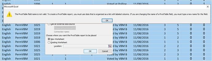
If you can’t read the Excel error, it reads, “The PivotTable field name is not valid. To create a PivotTable report, you must use data that is organized as a list with labeled columns. If you are changing the name of a PivotTable field, you must type a new name for the field.“
My solution came down to 2 separate problems.
Solution 1: Unhide Excel Columns
The spreadsheet I was using was extensive. It had 121 columns, and I hid many because I wasn’t using them. I decided to unhide all the columns to see if this was the only issue causing the error.
- Click the Select All button to the left of cell A1.
- Right-click any column heading and select Unhide.
- Try your Pivot Table again.
In my case, I still got the error.
Solution 2: Delete Empty Excel Columns
The next fix took a bit longer and did require I have all columns visible. This spreadsheet had some columns with headers but no values in any of the cells. Yes, that’s why I hid them.
In my case, I thought it would be easier to make a copy of my spreadsheet and then delete these columns. This way, I still had the original file.
It worked when I created my Pivot Table on the smaller working file.
See all How-To Articles
This tutorial demonstrates how to fix a pivot table field name that is not valid in Excel and Google Sheets.

Invalid Pivot Table Field Name
To create a pivot table in Excel, the data in your worksheet must be setup in a certain format. Excel does not like blank column names, or blank columns within its data! This tutorial troubleshoots some of the reasons for this error occurring.
Missing Column Names
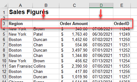
To create a pivot table, you need a row of column headers in the first row of your data. If any of the columns in the first row of your data is blank, you get an error message.
- Make sure you have column names in each cell of the first row.
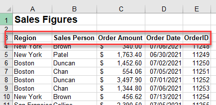
- Then try to create the pivot table again.
Blank Columns
Hidden blank columns can also cause the field name error.
Select the columns on either side of the hidden column or columns, right-click with the mouse, and then click Unhide to show the hidden columns.
Once the column is visible, right-click the column(s) and click Delete to remove the column.
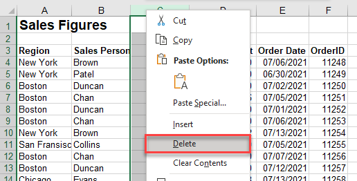
You can then try to insert your pivot table once again.
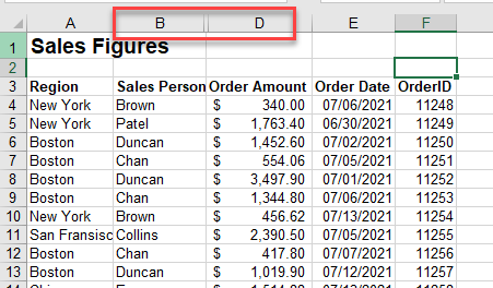
Merged Cells
If you have a heading with merged cells, you can get the field name error.
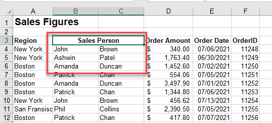
In the above example, although the Sales Person heading has been merged across Columns B and C, the actual names are separated into two columns.
To fix this, either:
Unmerge B3 and type in First Name and Surname;
OR
Concatenate the names together into one column and remove the merged header.
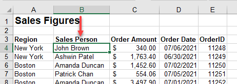
Then you can successfully insert a pivot table using the data.
Pivot Table Field Name Error in Google Sheets
Google Sheets is not as fussy as Excel when there are blank column names or hidden columns in a sheet. It creates the pivot table anyway. Then it is up to you as the user to make sure that the rows, columns, and values you insert into the pivot table return the correct data.
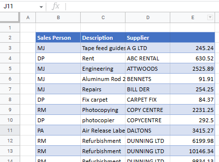
- In the following example, the data is laid out in a format that is compatible with creating a pivot table. However, there is no heading in cell E2.
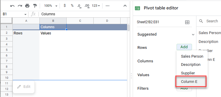
- When you create a pivot table with this data, Google Sheets just sets a field name (here, Column E) for the unnamed column; the other fields show up with their Row 2 headings.
- You can use the data in your pivot from the unnamed column as you would with a named column.
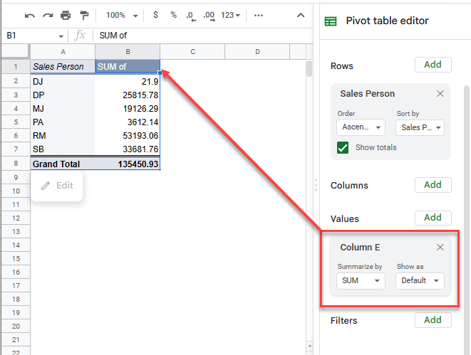
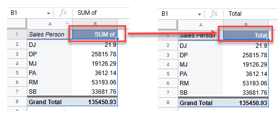
- The only “error” that occurs is that the column name is missing; the field shows only SUM of. To solve this problem, type your own name into the pivot field’s value header.
Tip: Try using some shortcuts when you’re working with pivot tables.